CBERS simulation from SPOT and its restoration
Gerald Jean Francis Banon and Leila Maria Garcia Fonseca
Content
1 CBERS Band 4 simulation from SPOT
1.1 Along line MTF of CBERS Band 4
1.2 Along line MTF of SPOT Band 3
1.3 Along line MTF of the simulation filter
1.4 Along line simulation filter kernel
1.5 MTF of the file effect
1.6 Along track MTF of CBERS Band 4
1.7 Along track MTF of SPOT Band 3
1.8 Along track MTF of the simulation filter
1.9 Along track simulation filter kernel
1.10 Simulation filter kernel
2 CBERS Band 4 Restoration
2.1 Along line MTF of the restoration filter
2.2 Along line restoration filter kernel
2.3 Along line MTF of the restored CBERS Band 4
2.4 Along track MTF of the restoration filter
2.5 Along track restoration filter kernel
2.6 Along track MTF of the restored CBERS Band 4
2.7 Restoration filter kernel
3 CBERS Band 4 Restoration using an Hanning window
3.1 Along line restoration filter kernel
3.2 Along line MTF of the restored CBERS Band 4
3.3 Along track restoration filter kernel
3.4 Along track MTF of the restored CBERS Band 4
3.5 Restoration filter kernel
4. Image pairs for comparison
4.1 Simulation
4.2 Restoration
Bibliography
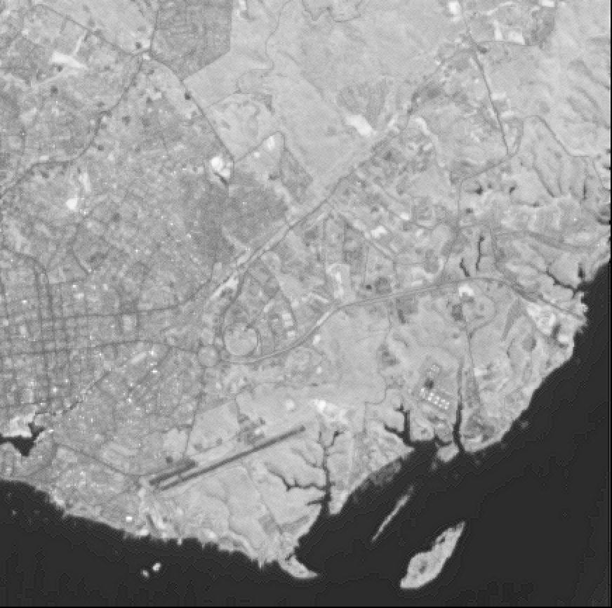
 SPOT Image
(contrast strech done using xv with point (152,255))
SPOT Image
(contrast strech done using xv with point (152,255))
 SPOT Image
(enlarged image - twice the original image in both directions)
(contrast strech done using xv with points (64,150) and (192,255))
1 CBERS SIMULATION FROM SPOT
1.1 ALONG LINE MTF OF CBERS BAND 4
function c=cbers1
f(1)=1;
f(2)=1;
f(3)=.98;
f(4)=.88;
f(5)=.70;
f(6)=.56;
f(7)=.42;
f(8)=.32;
f(9)=.28;
f(10)=.22;
f(11)=.18;
f(12)=.15;
f(13)=.12;
f(14)=.11;
f(15)=.085;
f(16)=.08;
f(17)=.075;
f(18)=.07;
f(19)=.065;
f(20)=.06;
for i=1:19
c(i+1)=f(i+1);
c(i+20)=f(21-i);
end
c(1)=f(1);
figure
x=cbers1;
plot(0:2:38,x(1:20))
xlabel('lp/mm')
title('Figure 1 - Along line MTF of CBERS Band 4')
see plot
EIFOV definition:
EIFOV=1/(2*MTF(.5))
From the along line MTF of CBERS Band 4, MTF(.5)=11 lp/mm
Let compute the EIFOV in m.
We assume that the earth sample interval is 19,5 m
and that the half sample frequency (from the MTF graph) is 38.5 lp/mm
EIFOV: 1/(2*11) 1/lp/mm <--> x m
1/38.5 1/lp/mm <--> 2*19.5 m
That is:
EIFOV=2*19.5*38.5/(2*11)=68.25 m
1.2 ALONG LINE MTF OF SPOT BAND 3
The MTF is gaussian with parameter sigma=11.2906 m
(Begni & Rayssiguiar, 1983)
1/(2*19.5) 1/m <--> 38.5 lp/mm
x 1/m <--> 38 lp/mm
38 lp/mm is chosen as the half sample frequency for the sake of
simplicity when computing later the Point Spread Function (PSF).
x=(38/38.5)/(2*19.5)
function s=spot1
N=19;
f(1)=1;
for n=1:19
u=(n/N)*(38/38.5)/(2*19.5);
f(n+1)=exp(-2*(3.1416^2)*(11.2906^2)*(u^2));
end
for i=1:19
s(i+1)=f(i+1);
s(i+20)=f(21-i);
end
s(1)=f(1);
x=spot1;
plot(0:2:38,x(1:20))
xlabel('lp/mm')
title('Figure 2 - Along line MTF of SPOT Band 3')
see plot
From the along line MTF of SPOT Band 3, MTF(.5)=25 lp/mm
That is:
EIFOV=2*19.5*38.5/(2*25)=30.03 m
Using the Gaussian assumption:
EIFOV=sigma*pi/((2*log(2))^.5)
EIFOV=11.2906*pi/((2*log(2))^.5)=30.1258 m
1.3 ALONG LINE MTF OF THE SIMULATION FILTER
function f=filter1
c=cbers1;
s=spot1;
for i=1:39
f(i)=c(i)/s(i);
end
x=filter1;
plot(0:2:38,x(1:20))
xlabel('lp/mm')
title('Figure 3 - Along line MTF of the simulation filter')
see plot
1.4 ALONG LINE SIMULATION FILTER KERNEL
x=real(fft(filter1,39));
plot(0:19,x(1:20))
xlabel('pixel')
title('Figure 4 - Along line PSF for the CBERS simulation')
see plot
function k=kernel1
x=real(fft(filter1,39));
k(1)=x(4);
k(2)=x(3);
k(3)=x(2);
k(4)=x(1);
k(5)=x(2);
k(6)=x(3);
k(7)=x(4);
a=0;
for i=1:7
a=a+k(i);
end
for i=1:7
k(i)=k(i)/a;
end
kernel1
0.0216 0.0944 0.1646 0.4391 0.1646 0.0944 0.0216
1.5 MTF OF THE FILE EFFECT
function s=file
N=19;
f(1)=1;
for n=1:19
u=(n/N)*(38/38.5)/(2*19.5);
f(n+1)=sin(3.1416*u*19.5)/(3.1416*u*19.5);
end
for i=1:19
s(i+1)=f(i+1);
s(i+20)=f(21-i);
end
s(1)=f(1);
x=file;
plot(0:2:38,x(1:20))
xlabel('lp/mm')
title('Figure 5 - MTF of the file effect')
see plot
1.6 ALONG TRACK MTF OF CBERS BAND 4
function f=cbers2
b=file;
c=cbers1;
for i=1:39
f(i)=b(i)*c(i);
end
x=cbers2;
plot(0:2:38,x(1:20))
xlabel('lp/mm')
title('Figure 6 - Along track MTF of CBERS Band 4')
see plot
From the along track MTF of CBERS Band 4, MTF(.5)=10.5 lp/mm
That is:
EIFOV=2*19.5*38.5/(2*10.5)=71.50 m
1.7 ALONG TRACK MTF OF SPOT BAND 3
The MTF is gaussian with parameter sigma = 10.3840 m
(Begni & Rayssiguiar, 1983)
function s=spot2
N=19;
f(1)=1;
for n=1:19
u=(n/N)*(38/38.5)/(2*19.5);
f(n+1)=exp(-2*(3.1416^2)*(10.3840^2)*(u^2));
end
for i=1:19
s(i+1)=f(i+1);
s(i+20)=f(21-i);
end
s(1)=f(1);
x=spot2;
plot(0:2:38,x(1:20))
xlabel('lp/mm')
title('Figure 7 - Along track MTF of SPOT Band 3')
see plot
From the along track MTF of SPOT Band 3, MTF(.5)=27 lp/mm
That is:
EIFOV=2*19.5*38.5/(2*27)=27.81 m
Using the Gaussian assumption:
EIFOV=10.3840*pi/((2*log(2))^.5)=27.7068 m
1.8 ALONG TRACK MTF OF THE SIMULATION FILTER
function f=filter2
b=file;
c=cbers1;
s=spot2;
for i=1:39
f(i)=b(i)*c(i)/s(i);
end
x=filter2;
plot(0:2:38,x(1:20))
xlabel('lp/mm')
title('Figure 8 - Along track MTF of the simulation filter')
see plot
1.9 ALONG TRACK SIMULATION FILTER KERNEL
x=real(fft(filter2,39));
plot(0:19,x(1:20))
xlabel('pixel')
title('Figure 9 - Along track PSF for the CBERS simulation')
see plot
function k=kernel2
x=real(fft(filter2,39));
k(1)=x(4);
k(2)=x(3);
k(3)=x(2);
k(4)=x(1);
k(5)=x(2);
k(6)=x(3);
k(7)=x(4);
a=0;
for i=1:7
a=a+k(i);
end
for i=1:7
k(i)=k(i)/a;
end
kernel2
0.0292 0.0885 0.1889 0.3868 0.1889 0.0885 0.0292
1.10 Simulation filter kernel
kernel2'*kernel1
0.0006 0.0028 0.0048 0.0128 0.0048 0.0028 0.0006
0.0019 0.0084 0.0146 0.0389 0.0146 0.0084 0.0019
0.0041 0.0178 0.0311 0.0829 0.0311 0.0178 0.0041
0.0083 0.0365 0.0637 0.1699 0.0637 0.0365 0.0083
0.0041 0.0178 0.0311 0.0829 0.0311 0.0178 0.0041
0.0019 0.0084 0.0146 0.0389 0.0146 0.0084 0.0019
0.0006 0.0028 0.0048 0.0128 0.0048 0.0028 0.0006
SPOT Image
(enlarged image - twice the original image in both directions)
(contrast strech done using xv with points (64,150) and (192,255))
1 CBERS SIMULATION FROM SPOT
1.1 ALONG LINE MTF OF CBERS BAND 4
function c=cbers1
f(1)=1;
f(2)=1;
f(3)=.98;
f(4)=.88;
f(5)=.70;
f(6)=.56;
f(7)=.42;
f(8)=.32;
f(9)=.28;
f(10)=.22;
f(11)=.18;
f(12)=.15;
f(13)=.12;
f(14)=.11;
f(15)=.085;
f(16)=.08;
f(17)=.075;
f(18)=.07;
f(19)=.065;
f(20)=.06;
for i=1:19
c(i+1)=f(i+1);
c(i+20)=f(21-i);
end
c(1)=f(1);
figure
x=cbers1;
plot(0:2:38,x(1:20))
xlabel('lp/mm')
title('Figure 1 - Along line MTF of CBERS Band 4')
see plot
EIFOV definition:
EIFOV=1/(2*MTF(.5))
From the along line MTF of CBERS Band 4, MTF(.5)=11 lp/mm
Let compute the EIFOV in m.
We assume that the earth sample interval is 19,5 m
and that the half sample frequency (from the MTF graph) is 38.5 lp/mm
EIFOV: 1/(2*11) 1/lp/mm <--> x m
1/38.5 1/lp/mm <--> 2*19.5 m
That is:
EIFOV=2*19.5*38.5/(2*11)=68.25 m
1.2 ALONG LINE MTF OF SPOT BAND 3
The MTF is gaussian with parameter sigma=11.2906 m
(Begni & Rayssiguiar, 1983)
1/(2*19.5) 1/m <--> 38.5 lp/mm
x 1/m <--> 38 lp/mm
38 lp/mm is chosen as the half sample frequency for the sake of
simplicity when computing later the Point Spread Function (PSF).
x=(38/38.5)/(2*19.5)
function s=spot1
N=19;
f(1)=1;
for n=1:19
u=(n/N)*(38/38.5)/(2*19.5);
f(n+1)=exp(-2*(3.1416^2)*(11.2906^2)*(u^2));
end
for i=1:19
s(i+1)=f(i+1);
s(i+20)=f(21-i);
end
s(1)=f(1);
x=spot1;
plot(0:2:38,x(1:20))
xlabel('lp/mm')
title('Figure 2 - Along line MTF of SPOT Band 3')
see plot
From the along line MTF of SPOT Band 3, MTF(.5)=25 lp/mm
That is:
EIFOV=2*19.5*38.5/(2*25)=30.03 m
Using the Gaussian assumption:
EIFOV=sigma*pi/((2*log(2))^.5)
EIFOV=11.2906*pi/((2*log(2))^.5)=30.1258 m
1.3 ALONG LINE MTF OF THE SIMULATION FILTER
function f=filter1
c=cbers1;
s=spot1;
for i=1:39
f(i)=c(i)/s(i);
end
x=filter1;
plot(0:2:38,x(1:20))
xlabel('lp/mm')
title('Figure 3 - Along line MTF of the simulation filter')
see plot
1.4 ALONG LINE SIMULATION FILTER KERNEL
x=real(fft(filter1,39));
plot(0:19,x(1:20))
xlabel('pixel')
title('Figure 4 - Along line PSF for the CBERS simulation')
see plot
function k=kernel1
x=real(fft(filter1,39));
k(1)=x(4);
k(2)=x(3);
k(3)=x(2);
k(4)=x(1);
k(5)=x(2);
k(6)=x(3);
k(7)=x(4);
a=0;
for i=1:7
a=a+k(i);
end
for i=1:7
k(i)=k(i)/a;
end
kernel1
0.0216 0.0944 0.1646 0.4391 0.1646 0.0944 0.0216
1.5 MTF OF THE FILE EFFECT
function s=file
N=19;
f(1)=1;
for n=1:19
u=(n/N)*(38/38.5)/(2*19.5);
f(n+1)=sin(3.1416*u*19.5)/(3.1416*u*19.5);
end
for i=1:19
s(i+1)=f(i+1);
s(i+20)=f(21-i);
end
s(1)=f(1);
x=file;
plot(0:2:38,x(1:20))
xlabel('lp/mm')
title('Figure 5 - MTF of the file effect')
see plot
1.6 ALONG TRACK MTF OF CBERS BAND 4
function f=cbers2
b=file;
c=cbers1;
for i=1:39
f(i)=b(i)*c(i);
end
x=cbers2;
plot(0:2:38,x(1:20))
xlabel('lp/mm')
title('Figure 6 - Along track MTF of CBERS Band 4')
see plot
From the along track MTF of CBERS Band 4, MTF(.5)=10.5 lp/mm
That is:
EIFOV=2*19.5*38.5/(2*10.5)=71.50 m
1.7 ALONG TRACK MTF OF SPOT BAND 3
The MTF is gaussian with parameter sigma = 10.3840 m
(Begni & Rayssiguiar, 1983)
function s=spot2
N=19;
f(1)=1;
for n=1:19
u=(n/N)*(38/38.5)/(2*19.5);
f(n+1)=exp(-2*(3.1416^2)*(10.3840^2)*(u^2));
end
for i=1:19
s(i+1)=f(i+1);
s(i+20)=f(21-i);
end
s(1)=f(1);
x=spot2;
plot(0:2:38,x(1:20))
xlabel('lp/mm')
title('Figure 7 - Along track MTF of SPOT Band 3')
see plot
From the along track MTF of SPOT Band 3, MTF(.5)=27 lp/mm
That is:
EIFOV=2*19.5*38.5/(2*27)=27.81 m
Using the Gaussian assumption:
EIFOV=10.3840*pi/((2*log(2))^.5)=27.7068 m
1.8 ALONG TRACK MTF OF THE SIMULATION FILTER
function f=filter2
b=file;
c=cbers1;
s=spot2;
for i=1:39
f(i)=b(i)*c(i)/s(i);
end
x=filter2;
plot(0:2:38,x(1:20))
xlabel('lp/mm')
title('Figure 8 - Along track MTF of the simulation filter')
see plot
1.9 ALONG TRACK SIMULATION FILTER KERNEL
x=real(fft(filter2,39));
plot(0:19,x(1:20))
xlabel('pixel')
title('Figure 9 - Along track PSF for the CBERS simulation')
see plot
function k=kernel2
x=real(fft(filter2,39));
k(1)=x(4);
k(2)=x(3);
k(3)=x(2);
k(4)=x(1);
k(5)=x(2);
k(6)=x(3);
k(7)=x(4);
a=0;
for i=1:7
a=a+k(i);
end
for i=1:7
k(i)=k(i)/a;
end
kernel2
0.0292 0.0885 0.1889 0.3868 0.1889 0.0885 0.0292
1.10 Simulation filter kernel
kernel2'*kernel1
0.0006 0.0028 0.0048 0.0128 0.0048 0.0028 0.0006
0.0019 0.0084 0.0146 0.0389 0.0146 0.0084 0.0019
0.0041 0.0178 0.0311 0.0829 0.0311 0.0178 0.0041
0.0083 0.0365 0.0637 0.1699 0.0637 0.0365 0.0083
0.0041 0.0178 0.0311 0.0829 0.0311 0.0178 0.0041
0.0019 0.0084 0.0146 0.0389 0.0146 0.0084 0.0019
0.0006 0.0028 0.0048 0.0128 0.0048 0.0028 0.0006
 Simulated CBERS Image
(contrast strech done using xv with point (152,255))
Simulated CBERS Image
(contrast strech done using xv with point (152,255))
 Simulated CBERS Image
(enlarged image - twice the original image in both directions)
2 CBERS BAND 4 RESTORATION
2.1 ALONG LINE MTF OF THE RESTORATION FILTER
In this secftion, the restoration objective is to return to the
SPOT Band 3 along line MTF
function r=restoration1
c=cbers1;
s=spot1;
for i=1:39
r(i)=s(i)/c(i);
end
x=restoration1;
plot(0:2:38,x(1:20))
xlabel('lp/mm')
title('Figure 10 - Along line MTF of the restoration filter')
see plot
2.2 ALONG LINE RESTORATION FILTER KERNEL
x=real(fft(restoration1,39));
plot(0:19,x(1:20))
xlabel('pixel')
title('Figure 11 - Along line PSF for the CBERS restoration')
see plot
function k=kernelForRestoration1
x=real(fft(restoration1,39));
k(1)=x(4);
k(2)=x(3);
k(3)=x(2);
k(4)=x(1);
k(5)=x(2);
k(6)=x(3);
k(7)=x(4);
a=0;
for i=1:7
a=a+k(i);
end
for i=1:7
k(i)=k(i)/a;
end
kernelForRestoration1
0.1907 -0.3224 -0.8181 2.8997 -0.8181 -0.3224 0.1907
2.3 ALONG LINE MTF OF THE RESTORED CBERS BAND 4
function h=restoredCBERSMTF1;
% Filter size = N*2+1
% Filter coefficients are truncated
N=4;
x=real(fft(restoration1,39));
for i=1:N
f(i)=x(i);
end
for i=N+1:20
f(i)=0;
end
for i=1:19
c(i+1)=f(i+1);
c(i+20)=f(21-i);
end
c(1)=f(1);
r=real(fft(c,39));
c=cbers1;
for i=1:39
g(i)=c(i)*r(i);
end
for i=1:39
h(i)=g(i)/g(1);
end
x=restoredCBERSMTF1;
plot(0:2:38,x(1:20))
xlabel('lp/mm')
title('Figure 12 - Along line MTF of the restored CBERS Band 4')
see plot
2.4 ALONG TRACK MTF OF THE RESTORATION FILTER
In this section, the restoration objective is to return to the
SPOT Band 3 along track MTF
function r=restoration2
c=cbers2;
s=spot2;
for i=1:39
r(i)=s(i)/c(i);
end
x=restoration2;
plot(0:2:38,x(1:20))
xlabel('lp/mm')
title('Figure 13 - Along track MTF of the restoration filter')
see plot
2.5 ALONG TRACK RESTORATION FILTER KERNEL
x=real(fft(restoration2,39));
plot(0:19,x(1:20))
xlabel('pixel')
title('Figure 14 - Along track PSF for the CBERS restoration')
see plot
function k=kernelForRestoration2
x=real(fft(restoration2,39));
k(1)=x(4);
k(2)=x(3);
k(3)=x(2);
k(4)=x(1);
k(5)=x(2);
k(6)=x(3);
k(7)=x(4);
a=0;
for i=1:7
a=a+k(i);
end
for i=1:7
k(i)=k(i)/a;
end
kernelForRestoration2
0.1694 -0.0908 -1.5746 3.9920 -1.5746 -0.0908 0.1694
2.6 ALONG TRACK MTF OF THE RESTORED CBERS BAND 4
function h=restoredCBERSMTF2;
% Filter size = N*2+1
% Filter coefficients are truncated
N=4;
x=real(fft(restoration2,39));
for i=1:N
f(i)=x(i);
end
for i=N+1:20
f(i)=0;
end
for i=1:19
c(i+1)=f(i+1);
c(i+20)=f(21-i);
end
c(1)=f(1);
r=real(fft(c,39));
c=cbers2;
for i=1:39
g(i)=c(i)*r(i);
end
for i=1:39
h(i)=g(i)/g(1);
end
x=restoredCBERSMTF2;
plot(0:2:38,x(1:20))
xlabel('lp/mm')
title('Figure 15 - Along track MTF of the restored CBERS Band 4')
see plot
2.7 RESTORATION FILTER KERNEL
kernelForRestoration2'*kernelForRestoration1
0.0323 -0.0546 -0.1386 0.4912 -0.1386 -0.0546 0.0323
-0.0173 0.0293 0.0743 -0.2633 0.0743 0.0293 -0.0173
-0.3002 0.5076 1.2882 -4.5660 1.2882 0.5076 -0.3002
0.7611 -1.2870 -3.2660 11.5758 -3.2660 -1.2870 0.7611
-0.3002 0.5076 1.2882 -4.5660 1.2882 0.5076 -0.3002
-0.0173 0.0293 0.0743 -0.2633 0.0743 0.0293 -0.0173
0.0323 -0.0546 -0.1386 0.4912 -0.1386 -0.0546 0.0323
Simulated CBERS Image
(enlarged image - twice the original image in both directions)
2 CBERS BAND 4 RESTORATION
2.1 ALONG LINE MTF OF THE RESTORATION FILTER
In this secftion, the restoration objective is to return to the
SPOT Band 3 along line MTF
function r=restoration1
c=cbers1;
s=spot1;
for i=1:39
r(i)=s(i)/c(i);
end
x=restoration1;
plot(0:2:38,x(1:20))
xlabel('lp/mm')
title('Figure 10 - Along line MTF of the restoration filter')
see plot
2.2 ALONG LINE RESTORATION FILTER KERNEL
x=real(fft(restoration1,39));
plot(0:19,x(1:20))
xlabel('pixel')
title('Figure 11 - Along line PSF for the CBERS restoration')
see plot
function k=kernelForRestoration1
x=real(fft(restoration1,39));
k(1)=x(4);
k(2)=x(3);
k(3)=x(2);
k(4)=x(1);
k(5)=x(2);
k(6)=x(3);
k(7)=x(4);
a=0;
for i=1:7
a=a+k(i);
end
for i=1:7
k(i)=k(i)/a;
end
kernelForRestoration1
0.1907 -0.3224 -0.8181 2.8997 -0.8181 -0.3224 0.1907
2.3 ALONG LINE MTF OF THE RESTORED CBERS BAND 4
function h=restoredCBERSMTF1;
% Filter size = N*2+1
% Filter coefficients are truncated
N=4;
x=real(fft(restoration1,39));
for i=1:N
f(i)=x(i);
end
for i=N+1:20
f(i)=0;
end
for i=1:19
c(i+1)=f(i+1);
c(i+20)=f(21-i);
end
c(1)=f(1);
r=real(fft(c,39));
c=cbers1;
for i=1:39
g(i)=c(i)*r(i);
end
for i=1:39
h(i)=g(i)/g(1);
end
x=restoredCBERSMTF1;
plot(0:2:38,x(1:20))
xlabel('lp/mm')
title('Figure 12 - Along line MTF of the restored CBERS Band 4')
see plot
2.4 ALONG TRACK MTF OF THE RESTORATION FILTER
In this section, the restoration objective is to return to the
SPOT Band 3 along track MTF
function r=restoration2
c=cbers2;
s=spot2;
for i=1:39
r(i)=s(i)/c(i);
end
x=restoration2;
plot(0:2:38,x(1:20))
xlabel('lp/mm')
title('Figure 13 - Along track MTF of the restoration filter')
see plot
2.5 ALONG TRACK RESTORATION FILTER KERNEL
x=real(fft(restoration2,39));
plot(0:19,x(1:20))
xlabel('pixel')
title('Figure 14 - Along track PSF for the CBERS restoration')
see plot
function k=kernelForRestoration2
x=real(fft(restoration2,39));
k(1)=x(4);
k(2)=x(3);
k(3)=x(2);
k(4)=x(1);
k(5)=x(2);
k(6)=x(3);
k(7)=x(4);
a=0;
for i=1:7
a=a+k(i);
end
for i=1:7
k(i)=k(i)/a;
end
kernelForRestoration2
0.1694 -0.0908 -1.5746 3.9920 -1.5746 -0.0908 0.1694
2.6 ALONG TRACK MTF OF THE RESTORED CBERS BAND 4
function h=restoredCBERSMTF2;
% Filter size = N*2+1
% Filter coefficients are truncated
N=4;
x=real(fft(restoration2,39));
for i=1:N
f(i)=x(i);
end
for i=N+1:20
f(i)=0;
end
for i=1:19
c(i+1)=f(i+1);
c(i+20)=f(21-i);
end
c(1)=f(1);
r=real(fft(c,39));
c=cbers2;
for i=1:39
g(i)=c(i)*r(i);
end
for i=1:39
h(i)=g(i)/g(1);
end
x=restoredCBERSMTF2;
plot(0:2:38,x(1:20))
xlabel('lp/mm')
title('Figure 15 - Along track MTF of the restored CBERS Band 4')
see plot
2.7 RESTORATION FILTER KERNEL
kernelForRestoration2'*kernelForRestoration1
0.0323 -0.0546 -0.1386 0.4912 -0.1386 -0.0546 0.0323
-0.0173 0.0293 0.0743 -0.2633 0.0743 0.0293 -0.0173
-0.3002 0.5076 1.2882 -4.5660 1.2882 0.5076 -0.3002
0.7611 -1.2870 -3.2660 11.5758 -3.2660 -1.2870 0.7611
-0.3002 0.5076 1.2882 -4.5660 1.2882 0.5076 -0.3002
-0.0173 0.0293 0.0743 -0.2633 0.0743 0.0293 -0.0173
0.0323 -0.0546 -0.1386 0.4912 -0.1386 -0.0546 0.0323
 Restored CBERS Image
(contrast strech done using xv with point (152,255))
Restored CBERS Image
(contrast strech done using xv with point (152,255))
 Restored CBERS Image
(enlarged image - twice the original image in both directions)
3 CBERS BAND 4 RESTORATION USING AN HANNING WINDOW
3.1 ALONG LINE RESTORATION FILTER KERNEL
function g=restorationKernel1;
% Filter size = N*2+1
% Filter coefficients are truncated by Hanning window
N=4;
x=real(fft(restoration1,39));
for i=1:N
f(i)=x(i)*(0.5+0.5*cos(3.141592*(i-1)/(N)));
end
s=0.;
for i=2:N
s=s+2*f(i);
end;
s=s+f(1);
for i=1:N
f(i)=f(i)/s;
end;
j=1;
for i=2:N
g(j+N)=f(i);
g(j)=f(N-i+2);
j=j+1;
end;
g(N)=f(1);
restorationKernel1
0.0226 -0.1304 -0.5647 2.3450 -0.5647 -0.1304 0.0226
3.2 ALONG LINE MTF OF THE RESTORED CBERS BAND 4
function h=restoredCBERSMTFh1;
% Filter size = N*2+1
% Filter coefficients are truncated by Hanning window
N=4;
x=real(fft(restoration1,39));
for i=1:N
f(i)=x(i)*(0.5+0.5*cos(3.141592*(i-1)/(N)));
end
for i=N+1:20
f(i)=0;
end
for i=1:19
c(i+1)=f(i+1);
c(i+20)=f(21-i);
end
c(1)=f(1);
r=real(fft(c,39));
c=cbers1;
for i=1:39
g(i)=c(i)*r(i);
end
for i=1:39
h(i)=g(i)/g(1);
end
x=restoredCBERSMTFh1;
plot(0:2:38,x(1:20))
xlabel('lp/mm')
title('Figure 16 - Along line MTF of the restored CBERS Band 4 (using an Hanning window)')
see plot
From the along line MTF of the restored CBERS Band 4, MTF(.5)=19.17 lp/mm
That is:
EIFOV=2*19.5*38.5/(2*19.17)=38.90 m
3.3 ALONG TRACK RESTORATION FILTER KERNEL
function g=restorationKernel2;
% Filter size = N*2+1
% Filter coefficients are truncated by Hanning window
N=4;
x=real(fft(restoration2,39));
for i=1:N
f(i)=x(i)*(0.5+0.5*cos(3.141592*(i-1)/(N)));
end
s=0.;
for i=2:N
s=s+2*f(i);
end;
s=s+f(1);
for i=1:N
f(i)=f(i)/s;
end;
j=1;
for i=2:N
g(j+N)=f(i);
g(j)=f(N-i+2);
j=j+1;
end;
g(N)=f(1);
restorationKernel2
0.0196 -0.0360 -1.0643 3.1613 -1.0643 -0.0360 0.0196
3.4 ALONG TRACK MTF OF THE RESTORED CBERS BAND 4
function h=restoredCBERSMTFh2;
% Filter size = N*2+1
% Filter coefficients are truncated by Hanning window
N=4;
x=real(fft(restoration2,39));
for i=1:N
f(i)=x(i)*(0.5+0.5*cos(3.141592*(i-1)/(N)));
end
for i=N+1:20
f(i)=0;
end
for i=1:19
c(i+1)=f(i+1);
c(i+20)=f(21-i);
end
c(1)=f(1);
r=real(fft(c,39));
c=cbers2;
for i=1:39
g(i)=c(i)*r(i);
end
for i=1:39
h(i)=g(i)/g(1);
end
x=restoredCBERSMTFh2;
plot(0:2:38,x(1:20))
xlabel('lp/mm')
title('Figure 17 - Along track MTF of the restored CBERS Band 4 (using an Hanning window)')
see plot
From the along track MTF of the restored CBERS Band 4, MTF(.5)=21.25 lp/mm
That is:
EIFOV=2*19.5*38.5/(2*21.25)=34.44 m
3.5 RESTORATION FILTER KERNEL
restorationKernel2'*restorationKernel1
0.0004 -0.0026 -0.0111 0.0461 -0.0111 -0.0026 0.0004
-0.0008 0.0047 0.0203 -0.0843 0.0203 0.0047 -0.0008
-0.0240 0.1387 0.6011 -2.4959 0.6011 0.1387 -0.0240
0.0714 -0.4121 -1.7852 7.4132 -1.7852 -0.4121 0.0714
-0.0240 0.1387 0.6011 -2.4959 0.6011 0.1387 -0.0240
-0.0008 0.0047 0.0203 -0.0843 0.0203 0.0047 -0.0008
0.0004 -0.0026 -0.0111 0.0461 -0.0111 -0.0026 0.0004
Restored CBERS Image
(enlarged image - twice the original image in both directions)
3 CBERS BAND 4 RESTORATION USING AN HANNING WINDOW
3.1 ALONG LINE RESTORATION FILTER KERNEL
function g=restorationKernel1;
% Filter size = N*2+1
% Filter coefficients are truncated by Hanning window
N=4;
x=real(fft(restoration1,39));
for i=1:N
f(i)=x(i)*(0.5+0.5*cos(3.141592*(i-1)/(N)));
end
s=0.;
for i=2:N
s=s+2*f(i);
end;
s=s+f(1);
for i=1:N
f(i)=f(i)/s;
end;
j=1;
for i=2:N
g(j+N)=f(i);
g(j)=f(N-i+2);
j=j+1;
end;
g(N)=f(1);
restorationKernel1
0.0226 -0.1304 -0.5647 2.3450 -0.5647 -0.1304 0.0226
3.2 ALONG LINE MTF OF THE RESTORED CBERS BAND 4
function h=restoredCBERSMTFh1;
% Filter size = N*2+1
% Filter coefficients are truncated by Hanning window
N=4;
x=real(fft(restoration1,39));
for i=1:N
f(i)=x(i)*(0.5+0.5*cos(3.141592*(i-1)/(N)));
end
for i=N+1:20
f(i)=0;
end
for i=1:19
c(i+1)=f(i+1);
c(i+20)=f(21-i);
end
c(1)=f(1);
r=real(fft(c,39));
c=cbers1;
for i=1:39
g(i)=c(i)*r(i);
end
for i=1:39
h(i)=g(i)/g(1);
end
x=restoredCBERSMTFh1;
plot(0:2:38,x(1:20))
xlabel('lp/mm')
title('Figure 16 - Along line MTF of the restored CBERS Band 4 (using an Hanning window)')
see plot
From the along line MTF of the restored CBERS Band 4, MTF(.5)=19.17 lp/mm
That is:
EIFOV=2*19.5*38.5/(2*19.17)=38.90 m
3.3 ALONG TRACK RESTORATION FILTER KERNEL
function g=restorationKernel2;
% Filter size = N*2+1
% Filter coefficients are truncated by Hanning window
N=4;
x=real(fft(restoration2,39));
for i=1:N
f(i)=x(i)*(0.5+0.5*cos(3.141592*(i-1)/(N)));
end
s=0.;
for i=2:N
s=s+2*f(i);
end;
s=s+f(1);
for i=1:N
f(i)=f(i)/s;
end;
j=1;
for i=2:N
g(j+N)=f(i);
g(j)=f(N-i+2);
j=j+1;
end;
g(N)=f(1);
restorationKernel2
0.0196 -0.0360 -1.0643 3.1613 -1.0643 -0.0360 0.0196
3.4 ALONG TRACK MTF OF THE RESTORED CBERS BAND 4
function h=restoredCBERSMTFh2;
% Filter size = N*2+1
% Filter coefficients are truncated by Hanning window
N=4;
x=real(fft(restoration2,39));
for i=1:N
f(i)=x(i)*(0.5+0.5*cos(3.141592*(i-1)/(N)));
end
for i=N+1:20
f(i)=0;
end
for i=1:19
c(i+1)=f(i+1);
c(i+20)=f(21-i);
end
c(1)=f(1);
r=real(fft(c,39));
c=cbers2;
for i=1:39
g(i)=c(i)*r(i);
end
for i=1:39
h(i)=g(i)/g(1);
end
x=restoredCBERSMTFh2;
plot(0:2:38,x(1:20))
xlabel('lp/mm')
title('Figure 17 - Along track MTF of the restored CBERS Band 4 (using an Hanning window)')
see plot
From the along track MTF of the restored CBERS Band 4, MTF(.5)=21.25 lp/mm
That is:
EIFOV=2*19.5*38.5/(2*21.25)=34.44 m
3.5 RESTORATION FILTER KERNEL
restorationKernel2'*restorationKernel1
0.0004 -0.0026 -0.0111 0.0461 -0.0111 -0.0026 0.0004
-0.0008 0.0047 0.0203 -0.0843 0.0203 0.0047 -0.0008
-0.0240 0.1387 0.6011 -2.4959 0.6011 0.1387 -0.0240
0.0714 -0.4121 -1.7852 7.4132 -1.7852 -0.4121 0.0714
-0.0240 0.1387 0.6011 -2.4959 0.6011 0.1387 -0.0240
-0.0008 0.0047 0.0203 -0.0843 0.0203 0.0047 -0.0008
0.0004 -0.0026 -0.0111 0.0461 -0.0111 -0.0026 0.0004
 Restored CBERS Image (using an Hanning window)
(contrast strech done using xv with point (152,255))
Restored CBERS Image (using an Hanning window)
(contrast strech done using xv with point (152,255))
 Restored CBERS Image (using an Hanning window)
(enlarged image - twice the original image in both directions)
4. IMAGE PAIRS FOR COMPARISON
4.1 SIMULATION
left: SPOT Image
(contrast strech done using xv with point (152,255))
right: Simulated CBERS Image
(contrast strech done using xv with point (152,255))
4.2 RESTORATION
left: SPOT Image
(contrast strech done using xv with point (152,255))
right: Restored CBERS Image (using an Hanning window)
(contrast strech done using xv with point (152,255))
BIBLIOGRAPHY
@Article{Banon:1990:SIB,
author = "Banon, G",
title = "simulacao de imagens de baixa resolucao",
journal = "Controle & Automacao",
year = "1990",
volume = "2",
number = "3",
pages = "180-192",
month = "March",
note = "INPE-8900-PRE/899",
annote = "entry from dpi.inpe.br/banon/1997/12.04.09.59",
citationkey = "Banon:1990:SIB",
entrytype = "Article",
type = "PRE",
}
@TechReport{BanonSant:1993:DFD,
author = "Banon, Gerald Jean Francis and Santos, Ailton Cruz
dos",
title = "Digital filter design for sensor simulation
application to the Brazilian Remote Sensing
Satellite",
institution = "INPE",
year = "1993",
type = "RPQ",
address = "Sao Jose dos campos",
note = "INPE-5523-RPQ/665",
abstract = "Neste artigo, um modelo de interacao, entre um
sensor de baixa resolucao com largo campo de
visada a bordo de um satelite de observacao da
terra, e a superficie da terra e apresentado. O
sensor simulado e obtido atraves da composicao de
um algoritmo de simulacao digital por um sensor de
alta resolucao e menor campo de visada. Uma nova
tecnica de desenvolvimento de filtro digital e
proposto para aproximar um filtro Gaussiano ideal.
O filtro resultante pode ser implementado em
qualquer plataforma existente de processamento de
imagens. Finalmente, dois retahos de imagem, da
maneira que eles seriam produzidos pelo SSR
(Satelite de Sensoriamento Remoto) da MECB (Missao
Espacial Completa Brasileira) a partir de uma cena
LANDSAT-TM (Thematic Mapper) sao apresentadas como
exemplo..",
annote = "entry from dpi.inpe.br/banon/1997/12.04.09.59",
citationkey = "BanonSant:1993:DFD",
entrytype = "TechReport",
}
@Article{BegniRays:1983:SpBiQu,
author = "Begni, G. and Rayssiguier, M.",
title = "Sp\'ecifications et bilans de qualit\'e image du
syst\`eme SPOT",
journal = "Acta Astronautica",
year = "1983",
volume = "10",
number = "1",
pages = "37--42",
keywords = "spot specification, mtf.",
entrytype = "Article",
}
@MastersThesis{Fonseca:1988:RII,
author = "Fonseca, Leila Maria Garcia",
title = "Restauracao e interpolacao de imagens do satelite
Landsat por meio de tecnicas de projeto de filtros
FIR",
school = "ITA",
year = "1988",
address = "Sao Jose dos Campos",
month = "April",
note = "INPE-8898-TAE/898",
annote = "entry from dpi.inpe.br/banon/1997/12.04.09.59",
citationkey = "Fonseca:1988:RII",
entrytype = "MastersThesis",
program = "DPI",
type = "TAE",
}
@InProceedings{FonsecaBano::DTF,
author = "Fonseca, Leila Maria Garcia and Banon, Gerald Jean
Francis",
title = "Duas tecnicas de filtragem espacial para simular a
resolucao espacial ao Nadir do satelite de
sensoriamento remoto brasileiro",
booktitle = "Simposio Brasileiro de Computacao Grafica e
Processamento de Imagens, 2",
pages = "69-76",
month = "April",
note = "INPE-8023-PRE/023. 26-28 abr., Aguas de Lindoia,
BR.",
abstract = "Este trabalho apresenta duas tecnicas de filtragem
espacial para simular a resolucao espacial ao
nadir do Satelite de Sensoriamento Remoto
brasileiro (SSR). Estas duas tecnicas sao
avaliadas atraves da sua aplicacao na simulacao de
imagens MSS. Posteriormente, os filtros sao
aplicados para simular a banda 1 so SSR a partir
da banda 3 do TM. De um modo geral, os resultados
mostraram-se satisfatorios.",
annote = "entry from dpi.inpe.br/banon/1997/12.04.09.59",
citationkey = "FonsecaBano::DTF",
entrytype = "InProceedings",
type = "PRE",
}
@InProceedings{FonsecaMasc:1988:MCI,
author = "Fonseca, Leila Maria Garcia and Mascarenhas,
Nelson Delfino d'Avila",
title = "Method for combined image
interpolation-restoration through a fir filter
design technique",
booktitle = "International Congress of Photogrammetry and
Remote Sensing, 16",
year = "1988",
pages = "196-206",
organization = "ISPRS",
note = "INPE-4561-PRE/1302. 1-10 July, Kyoto, Japan.",
keywords = "processamento digital e correcoes, restauracao de
imagens, tm landsat, interpolacao, resolucao de
imagens, filtros, digital processing and
correction, image restoration, interpolation,
image resolution, filters",
abstract = "In digital image processing there is often a need
to interpolated an image. Examples occur in scale
magnification, image registration, geometric
correction, etc. On the other hand, this image can
be subjected to several sources of resolution
degradation and an improvement of this resolution
may be necessary. Therefore, this paper addresses
the problem of combining the interpolation and the
restoration in a single operation, thereby
reducing the computacional effort. This is done by
means of a 2D, separable, FIR filter. The ideal
low-pass FIR filter for interpolation is modified
to account for the restoration process. The
Modified Inverse Filter (MIF) is used for this
purpose. The proposed method is applied to the
interpolation-restoration of Landsat-5 Thematic
Mapper data. The later process takes into account
the degradation due to optics, detector and
electronic filtering. A comparison with the
parametric cubic convolution interpolation
technique is made.",
annote = "entry from dpi.inpe.br/banon/1997/12.04.09.59",
citationkey = "FonsecaMasc:1988:MCI",
entrytype = "InProceedings",
type = "PRE",
volume = "v.27, Part B3",
}
@InProceedings{FonsecaMascBano:1987:TRR,
author = "Fonseca, Leila Maria Garcia and Mascarenhas,
Nelson Delfino d'Avila and Banon, Gerald Jean
Francis",
title = "Tecnicas de restauracao para remostragem de
imagens do satelite Landsat-5",
booktitle = "Simposio Brasileiro de Telecomunicacoes, 5",
year = "1987",
pages = "204-208",
organization = "Sociedade Brasileira de Telecomunicaoes",
month = "June",
note = "INPE-4189-PRE/1076. 8-10 set., Campinas, BR.",
keywords = "processamento digital e correcoes, restauracao de
imagens, landsat-5, transformada de fourier,
digital processing and correction, image
restoration, thematic mappers (landsat)",
abstract = "Sao mostrados neste trabalho alguns resultados da
restauracao para reamostragem de imagens do TM
(Thematic Mapper), utilizando tecnicas no dominio
de Fourier. A imagem restaurada e comparada a
aimagem reamostrada com o interpolador de
convolucao cubica. A comparacao e feita
visualmente e atraves do perfil radiometrico de
uma linha da imagem.",
annote = "entry from dpi.inpe.br/banon/1997/12.04.09.59",
citationkey = "FonsecaMascBano:1987:TRR",
entrytype = "InProceedings",
type = "PRE",
}
@Article{FonsecaPrasMasc:1993:CIL,
author = "Fonseca, L. M. G. and Prasad, G. S. S. D. and
Mascarenhas, N. D. A.",
title = "Combined interpolation-restoration of landsat
images through FIR filter techniques",
journal = "International Journal Remote Sensing",
year = "1993",
volume = "14",
number = "13",
pages = "2547--2561",
}
@InProceedings{MascarenhasBanoFons:1990:SPB,
author = "Mascarenhas, Nelson Delfini D'Avila and Banon,
Gerald Jean Francis and Fonseca, Leila Maria
Garcia",
title = "SPOT panchromatic band simulation by linear
combination of multispectral bands",
booktitle = "Simposio Brasileiro de Sensoriamento Remoto, 6",
year = "1990",
pages = "181-187",
organization = "Instituto Nacional de Pesquisas Espaciais",
note = "INPE-5295-PRE/1658. 24-29 jul., Manaus, BR.",
keywords = "processamento digital e correcoes, spot (satelite
frances, sensores, sensors",
abstract = "A simulacao de uma de mais bandas de um sensor
multiespectral por combinacao de outras bandas
apresenta possibilidades atraentes. Por exemplo,
ela poderia diminuir a taxa de dados do canal de
comunicacao entre o satelite e a terra. Neste
trabalho, e feita uma analise da simulacao da
banda pancromatica do SPOT (degrada
espacialmente), por uma combinacao linear de
bandas multiespectrais. Dois metod sao usados para
a combinacao linear espectral: a) minimo quadrado
sem restricao e b) minimo quadrado com restricoes
de igualdade. Usando o segundo metodo mostra-se
que a relacao sinal-ruido da banda simulada ttende
a ser melhor que a relacao sinal-ruido de cada
banda multiespectal. Os resultados experimentais
incluem a simulacao espacial de uma banda
pancromatica degradada espacialmente, com uma
resolucao de 20 m, opara comparacao com a banda
simulada espectralmente. Esses resultados
demostram que uma estimativa razoavekl do ponto de
vista visual e numerico da banda pancromatica
degradada pode ser obtida.",
annote = "entry from dpi.inpe.br/banon/1997/12.04.09.59",
citationkey = "MascarenhasBanoFons:1990:SPB",
entrytype = "InProceedings",
type = "PRE",
}
@InProceedings{MascarenhasBanoFons:1991:SAP,
author = "Mascarenhas, Nelson Delfino D'Avila and Banon,
Gerald Jean Francis and Fonseca, Leila Maria
Garcia",
title = "Simulation of a panchormatic band by spectral
linear combination of multiespectral bands",
booktitle = "International Symposium on Remote Sensing of
Environment,24",
year = "1991",
organization = "ERIM",
note = "INPE-5293-PRE/1698. 27-31 May, Rio de Janeiro,
BR.",
abstract = "The simulation of one or more bands of a
multispectral sensor by combination of other bands
represents an attractive possibility. In this work
an anlysis of the spatially degraded SPOT
panchromatic band by linear combination of the
multispectral bands has been performed using least
squares methods. The results include 1) a
theoretical study of the signal to noise ratio of
the simulated band as compared with the
multispectral bands, and 2) experimental work
showing a numerically and visually reasonable
estimate of the pancromatic band.",
annote = "entry from dpi.inpe.br/banon/1997/12.04.09.59",
citationkey = "MascarenhasBanoFons:1991:SAP",
entrytype = "InProceedings",
type = "PRE",
}
@MastersThesis{Santos:1992:SIS,
author = "Santos, Ailton Cruz",
title = "Simulacao de Imagens de Sensores com Largo Campo
de Visada a partir de Imagens de Sensores com
menor Campo de Visada- O caso SSR/TM",
school = "Instituto Nacional de Pesquisas Espaciais",
year = "1992",
address = "Sao Jose dos Campos",
month = "March",
note = "INPE-5378-TDI/473",
keywords = "Campo de visada, filtro, processamento
de imagens, mapeador tematico (landsat), satelites
landsat, computerized simulation, field of view,
image enhancement, image processing, thematic
mappers (landsat), adaptive filters",
abstract = " Com este trabalho pretende-se a simulacao da
imagem bruta obtida por um sensor orbital com
largo campo de visada sob um modelo aproximado
para o Satelite de Sensoriamento Remoto (SSR) da
Missao Espacial completa brasileira (MECB), a
partir de um conjunto de imagens obtidas por um
sensor com menor campo de visada. No caso, usou-se
um conjunto de imagens obtidas pelo sensor
TM/Landsat, construidas com controle geometrico em
uma projecao cartografica e corrigidas com pontos
de controle. Utilizando-se um modelo da superficie
terrestre, sao determinados os pontos na
superficie correspondente a projecao do centro de
cada detentor (em coordenadas geodesicas-latitude
e longitude). Os valores dos pixels da imagem com
largo campo de visada sao calculados a partir dos
valores dos pixels da imagem TM vizinhos a estes
pontos. Este calculo e feito empregando-se um
filtro de simulacao adaptativo. Os resultados
mostram-se satisfatorios considerando-se o aspecto
geometrico sob o qual foi desenvolvido o presente
trabalho.",
annote = "entry from dpi.inpe.br/banon/1997/12.04.09.59",
citationkey = "Santos:1992:SIS",
entrytype = "MastersThesis",
program = "SER",
type = "TDI",
}
Restored CBERS Image (using an Hanning window)
(enlarged image - twice the original image in both directions)
4. IMAGE PAIRS FOR COMPARISON
4.1 SIMULATION
left: SPOT Image
(contrast strech done using xv with point (152,255))
right: Simulated CBERS Image
(contrast strech done using xv with point (152,255))
4.2 RESTORATION
left: SPOT Image
(contrast strech done using xv with point (152,255))
right: Restored CBERS Image (using an Hanning window)
(contrast strech done using xv with point (152,255))
BIBLIOGRAPHY
@Article{Banon:1990:SIB,
author = "Banon, G",
title = "simulacao de imagens de baixa resolucao",
journal = "Controle & Automacao",
year = "1990",
volume = "2",
number = "3",
pages = "180-192",
month = "March",
note = "INPE-8900-PRE/899",
annote = "entry from dpi.inpe.br/banon/1997/12.04.09.59",
citationkey = "Banon:1990:SIB",
entrytype = "Article",
type = "PRE",
}
@TechReport{BanonSant:1993:DFD,
author = "Banon, Gerald Jean Francis and Santos, Ailton Cruz
dos",
title = "Digital filter design for sensor simulation
application to the Brazilian Remote Sensing
Satellite",
institution = "INPE",
year = "1993",
type = "RPQ",
address = "Sao Jose dos campos",
note = "INPE-5523-RPQ/665",
abstract = "Neste artigo, um modelo de interacao, entre um
sensor de baixa resolucao com largo campo de
visada a bordo de um satelite de observacao da
terra, e a superficie da terra e apresentado. O
sensor simulado e obtido atraves da composicao de
um algoritmo de simulacao digital por um sensor de
alta resolucao e menor campo de visada. Uma nova
tecnica de desenvolvimento de filtro digital e
proposto para aproximar um filtro Gaussiano ideal.
O filtro resultante pode ser implementado em
qualquer plataforma existente de processamento de
imagens. Finalmente, dois retahos de imagem, da
maneira que eles seriam produzidos pelo SSR
(Satelite de Sensoriamento Remoto) da MECB (Missao
Espacial Completa Brasileira) a partir de uma cena
LANDSAT-TM (Thematic Mapper) sao apresentadas como
exemplo..",
annote = "entry from dpi.inpe.br/banon/1997/12.04.09.59",
citationkey = "BanonSant:1993:DFD",
entrytype = "TechReport",
}
@Article{BegniRays:1983:SpBiQu,
author = "Begni, G. and Rayssiguier, M.",
title = "Sp\'ecifications et bilans de qualit\'e image du
syst\`eme SPOT",
journal = "Acta Astronautica",
year = "1983",
volume = "10",
number = "1",
pages = "37--42",
keywords = "spot specification, mtf.",
entrytype = "Article",
}
@MastersThesis{Fonseca:1988:RII,
author = "Fonseca, Leila Maria Garcia",
title = "Restauracao e interpolacao de imagens do satelite
Landsat por meio de tecnicas de projeto de filtros
FIR",
school = "ITA",
year = "1988",
address = "Sao Jose dos Campos",
month = "April",
note = "INPE-8898-TAE/898",
annote = "entry from dpi.inpe.br/banon/1997/12.04.09.59",
citationkey = "Fonseca:1988:RII",
entrytype = "MastersThesis",
program = "DPI",
type = "TAE",
}
@InProceedings{FonsecaBano::DTF,
author = "Fonseca, Leila Maria Garcia and Banon, Gerald Jean
Francis",
title = "Duas tecnicas de filtragem espacial para simular a
resolucao espacial ao Nadir do satelite de
sensoriamento remoto brasileiro",
booktitle = "Simposio Brasileiro de Computacao Grafica e
Processamento de Imagens, 2",
pages = "69-76",
month = "April",
note = "INPE-8023-PRE/023. 26-28 abr., Aguas de Lindoia,
BR.",
abstract = "Este trabalho apresenta duas tecnicas de filtragem
espacial para simular a resolucao espacial ao
nadir do Satelite de Sensoriamento Remoto
brasileiro (SSR). Estas duas tecnicas sao
avaliadas atraves da sua aplicacao na simulacao de
imagens MSS. Posteriormente, os filtros sao
aplicados para simular a banda 1 so SSR a partir
da banda 3 do TM. De um modo geral, os resultados
mostraram-se satisfatorios.",
annote = "entry from dpi.inpe.br/banon/1997/12.04.09.59",
citationkey = "FonsecaBano::DTF",
entrytype = "InProceedings",
type = "PRE",
}
@InProceedings{FonsecaMasc:1988:MCI,
author = "Fonseca, Leila Maria Garcia and Mascarenhas,
Nelson Delfino d'Avila",
title = "Method for combined image
interpolation-restoration through a fir filter
design technique",
booktitle = "International Congress of Photogrammetry and
Remote Sensing, 16",
year = "1988",
pages = "196-206",
organization = "ISPRS",
note = "INPE-4561-PRE/1302. 1-10 July, Kyoto, Japan.",
keywords = "processamento digital e correcoes, restauracao de
imagens, tm landsat, interpolacao, resolucao de
imagens, filtros, digital processing and
correction, image restoration, interpolation,
image resolution, filters",
abstract = "In digital image processing there is often a need
to interpolated an image. Examples occur in scale
magnification, image registration, geometric
correction, etc. On the other hand, this image can
be subjected to several sources of resolution
degradation and an improvement of this resolution
may be necessary. Therefore, this paper addresses
the problem of combining the interpolation and the
restoration in a single operation, thereby
reducing the computacional effort. This is done by
means of a 2D, separable, FIR filter. The ideal
low-pass FIR filter for interpolation is modified
to account for the restoration process. The
Modified Inverse Filter (MIF) is used for this
purpose. The proposed method is applied to the
interpolation-restoration of Landsat-5 Thematic
Mapper data. The later process takes into account
the degradation due to optics, detector and
electronic filtering. A comparison with the
parametric cubic convolution interpolation
technique is made.",
annote = "entry from dpi.inpe.br/banon/1997/12.04.09.59",
citationkey = "FonsecaMasc:1988:MCI",
entrytype = "InProceedings",
type = "PRE",
volume = "v.27, Part B3",
}
@InProceedings{FonsecaMascBano:1987:TRR,
author = "Fonseca, Leila Maria Garcia and Mascarenhas,
Nelson Delfino d'Avila and Banon, Gerald Jean
Francis",
title = "Tecnicas de restauracao para remostragem de
imagens do satelite Landsat-5",
booktitle = "Simposio Brasileiro de Telecomunicacoes, 5",
year = "1987",
pages = "204-208",
organization = "Sociedade Brasileira de Telecomunicaoes",
month = "June",
note = "INPE-4189-PRE/1076. 8-10 set., Campinas, BR.",
keywords = "processamento digital e correcoes, restauracao de
imagens, landsat-5, transformada de fourier,
digital processing and correction, image
restoration, thematic mappers (landsat)",
abstract = "Sao mostrados neste trabalho alguns resultados da
restauracao para reamostragem de imagens do TM
(Thematic Mapper), utilizando tecnicas no dominio
de Fourier. A imagem restaurada e comparada a
aimagem reamostrada com o interpolador de
convolucao cubica. A comparacao e feita
visualmente e atraves do perfil radiometrico de
uma linha da imagem.",
annote = "entry from dpi.inpe.br/banon/1997/12.04.09.59",
citationkey = "FonsecaMascBano:1987:TRR",
entrytype = "InProceedings",
type = "PRE",
}
@Article{FonsecaPrasMasc:1993:CIL,
author = "Fonseca, L. M. G. and Prasad, G. S. S. D. and
Mascarenhas, N. D. A.",
title = "Combined interpolation-restoration of landsat
images through FIR filter techniques",
journal = "International Journal Remote Sensing",
year = "1993",
volume = "14",
number = "13",
pages = "2547--2561",
}
@InProceedings{MascarenhasBanoFons:1990:SPB,
author = "Mascarenhas, Nelson Delfini D'Avila and Banon,
Gerald Jean Francis and Fonseca, Leila Maria
Garcia",
title = "SPOT panchromatic band simulation by linear
combination of multispectral bands",
booktitle = "Simposio Brasileiro de Sensoriamento Remoto, 6",
year = "1990",
pages = "181-187",
organization = "Instituto Nacional de Pesquisas Espaciais",
note = "INPE-5295-PRE/1658. 24-29 jul., Manaus, BR.",
keywords = "processamento digital e correcoes, spot (satelite
frances, sensores, sensors",
abstract = "A simulacao de uma de mais bandas de um sensor
multiespectral por combinacao de outras bandas
apresenta possibilidades atraentes. Por exemplo,
ela poderia diminuir a taxa de dados do canal de
comunicacao entre o satelite e a terra. Neste
trabalho, e feita uma analise da simulacao da
banda pancromatica do SPOT (degrada
espacialmente), por uma combinacao linear de
bandas multiespectrais. Dois metod sao usados para
a combinacao linear espectral: a) minimo quadrado
sem restricao e b) minimo quadrado com restricoes
de igualdade. Usando o segundo metodo mostra-se
que a relacao sinal-ruido da banda simulada ttende
a ser melhor que a relacao sinal-ruido de cada
banda multiespectal. Os resultados experimentais
incluem a simulacao espacial de uma banda
pancromatica degradada espacialmente, com uma
resolucao de 20 m, opara comparacao com a banda
simulada espectralmente. Esses resultados
demostram que uma estimativa razoavekl do ponto de
vista visual e numerico da banda pancromatica
degradada pode ser obtida.",
annote = "entry from dpi.inpe.br/banon/1997/12.04.09.59",
citationkey = "MascarenhasBanoFons:1990:SPB",
entrytype = "InProceedings",
type = "PRE",
}
@InProceedings{MascarenhasBanoFons:1991:SAP,
author = "Mascarenhas, Nelson Delfino D'Avila and Banon,
Gerald Jean Francis and Fonseca, Leila Maria
Garcia",
title = "Simulation of a panchormatic band by spectral
linear combination of multiespectral bands",
booktitle = "International Symposium on Remote Sensing of
Environment,24",
year = "1991",
organization = "ERIM",
note = "INPE-5293-PRE/1698. 27-31 May, Rio de Janeiro,
BR.",
abstract = "The simulation of one or more bands of a
multispectral sensor by combination of other bands
represents an attractive possibility. In this work
an anlysis of the spatially degraded SPOT
panchromatic band by linear combination of the
multispectral bands has been performed using least
squares methods. The results include 1) a
theoretical study of the signal to noise ratio of
the simulated band as compared with the
multispectral bands, and 2) experimental work
showing a numerically and visually reasonable
estimate of the pancromatic band.",
annote = "entry from dpi.inpe.br/banon/1997/12.04.09.59",
citationkey = "MascarenhasBanoFons:1991:SAP",
entrytype = "InProceedings",
type = "PRE",
}
@MastersThesis{Santos:1992:SIS,
author = "Santos, Ailton Cruz",
title = "Simulacao de Imagens de Sensores com Largo Campo
de Visada a partir de Imagens de Sensores com
menor Campo de Visada- O caso SSR/TM",
school = "Instituto Nacional de Pesquisas Espaciais",
year = "1992",
address = "Sao Jose dos Campos",
month = "March",
note = "INPE-5378-TDI/473",
keywords = "Campo de visada, filtro, processamento
de imagens, mapeador tematico (landsat), satelites
landsat, computerized simulation, field of view,
image enhancement, image processing, thematic
mappers (landsat), adaptive filters",
abstract = " Com este trabalho pretende-se a simulacao da
imagem bruta obtida por um sensor orbital com
largo campo de visada sob um modelo aproximado
para o Satelite de Sensoriamento Remoto (SSR) da
Missao Espacial completa brasileira (MECB), a
partir de um conjunto de imagens obtidas por um
sensor com menor campo de visada. No caso, usou-se
um conjunto de imagens obtidas pelo sensor
TM/Landsat, construidas com controle geometrico em
uma projecao cartografica e corrigidas com pontos
de controle. Utilizando-se um modelo da superficie
terrestre, sao determinados os pontos na
superficie correspondente a projecao do centro de
cada detentor (em coordenadas geodesicas-latitude
e longitude). Os valores dos pixels da imagem com
largo campo de visada sao calculados a partir dos
valores dos pixels da imagem TM vizinhos a estes
pontos. Este calculo e feito empregando-se um
filtro de simulacao adaptativo. Os resultados
mostram-se satisfatorios considerando-se o aspecto
geometrico sob o qual foi desenvolvido o presente
trabalho.",
annote = "entry from dpi.inpe.br/banon/1997/12.04.09.59",
citationkey = "Santos:1992:SIS",
entrytype = "MastersThesis",
program = "SER",
type = "TDI",
}